
Even though the NHL season is in the midst of the Stanley Cup Playoffs, it’s not too early to think about the off-season festivities of the NHL draft and free agency. One of the unique features of the NHL is that it is the most cap constrictive sport. This is in part because of three features: (1) the presence of a hard salary cap, (2) the nature of guaranteed contracts and (3) limited and no-trade clauses. The combination of these three factors separate the NHL from other leagues, namely the MLB, NFL and NBA. Other leagues have mechanisms for restructuring contracts, the lack of guaranteed money and/or soft salary cap restrictions.
How this translates to differentiate the NHL from other leagues is that the salary cap is the great equalizer, which can empower or impoverish a franchise with a few decisions. Aside from the compliance buyouts offered in the wake of the previous CBA, there are limited options for a team to jettison a player signed to a bad contract. Teams that sign players to long-term, big money contracts are held most accountable in the NHL, with limited options of movement that can hamstring a franchise for years.
Thanks to war-on-ice.com, I was able to analyze the relationship between Corsi values (shots taken for/against while on the ice/off the ice) and annual contract values for players. First, I map the Corsi for (herein CF) and Corsi against (herein CA) values on a (x,y) plot. The size of the bubbles (for each player) are relative to the value of their contract.
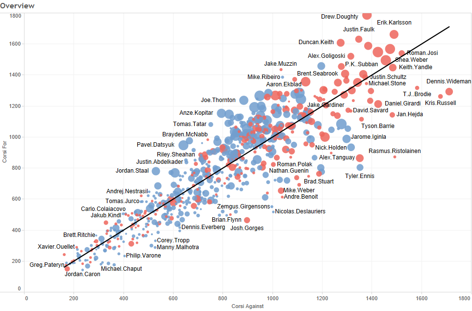
There are a few important observations one can extrapolate from this graph. For starters, the relationship between CF and CA is statistically significant at the P < .001 level. In other words, as the value of CF increases (meaning shots by your team, taken while said player is on the ice), so does the value of CA (shots taken against team, while said player is on the ice), There is a clustering in the middle of the graph, which means that most players are on the ice for roughly the same number of shots for and shots against. That being said, there are a few players that defy this logic, generating relatively significant shots for or against while on the ice. These players often have their names listed and include players that excel at CF, including Datsyuk, Kopitar, Thorton, Staal, Keith, Faulk, Karlsson and Doughty. Others are marred by high CA scores, including Wideman, Russell, Brodie, Hejda, Ennis and Gorges. Any player north of the black line has a positive Corsi score (CF-CA), and any player south of the black line has a negative Corsi score. That is not to say the Corsi statistics, sometimes treated as a magic bullet by the NHL analytic community, is a perfect measure of worth. It does illustrate puck possession, which is a large factor (albeit not the only one) in NHL success. In order to show the difference between forwards and defense, I have filtered the chart below:


One of the other facets of these graphs is the annual contract value of the player, illustrated by the size of the player bubble. It is quite interesting that most of the highest payed players exhibit positive corsi scores. There are exceptions, notably teammates Phaneuf and Kessel, who are making 7 Million and 8 Million respectively, yet whose Corsi differentials were both over -200. On the other end of the spectrum, Leddy, Jones and Ekblad made collectively less than 5 million, and posted admirably high Corsi scores.
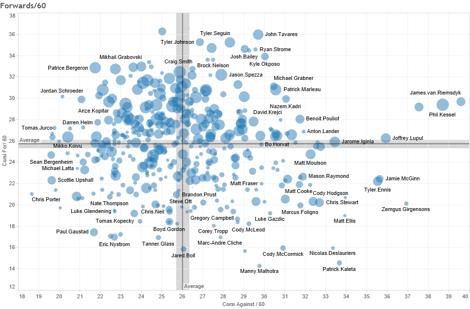
One of the downsides of looking at CF and CA scores is the sample size, which only takes into account 5v5 even strength play. Due to TOI (time on ice), limited by scratch or game situations, it does not standardize every player on the same scale. In order to achieve this, I standardize CA and CF if the player had played 60 minutes (which is obviously impossible), in order to differentiate those with wildly different TOI. The overview and the defense and forwards charts are below.
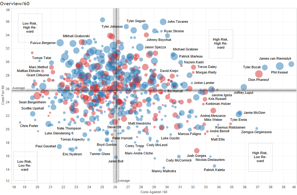

What is intriguing about graphing CA/60 and CF/60 is that four quadrants appear when the means and confidence intervals of the variables are applied. This illustrates the risk and reward of having these players on the ice. Depending on the game situation (leading, behind, close) certain players may be used for their strengths. It is no coincidence that a players like Bergeron and Kopitar are both in the top left corner, because of their low CA/60 and high CF/60 values. While Benn, Seguin and Tavares are in the top right, because they are less responsible in the shots against/60 category, but are also more prone to producing shots while on the ice. As one might expect, all of these players are fairly compensated for their performance on the ice.
To get right to the point, the last analysis uses the contract value as the x-axis and CF% (which is derived from CF/CA) as the y. The size of the bubbles represent TOI. The range of CF% per salary is astounding, such as Boychuk and Gorges having nearly the identical salary, yet polar opposite values of CF%.

In short, this exercise was to illustrate the importance of spending money wisely in the NHL. It is no coincidence that the teams who got the greatest value for their money are perennial cup contenders. Since the salary cap is a zero-sum game, the evaluation of free agents and not overpaying for mediocrity is essential to NHL success.
